Use of Arcpad to Deploy Projects into the Field

Introduction:

This week’s exercise involves the use of Arcpad integrated with Arcmap and the use of Trimble Juno GPS units.  Andrew Peterson, Amy Bartel and I worked together during this project to decide what data to collect, what attributes pertaining to that data would should be gathered and gathering the data.

Study area:

The data were gathered at the Priory and the immediate surrounding area. The Priory is located approximately 5 kilometers south of the University of Wisconsin Eau Claire (UWEC) campus on Priory Road. Directions to the Priory from UWEC are as follows. From the main campus area take Roosevelt Avenue east to State Street, turn right on State Street and follow it south until you come to Lowes Creek Road, turn right on West Lowes Creek Road, you will cross over Interstate 94 then come to Priory Road, turn right on Priory Road and watch for the sign for the Priory on your right. The terrain at the Priory consists of two levels of relatively flat ground connected with steep hills; the lower level has deep ravines cutting through it. The Priory sits on the top level of the property, a fairly flat topped hill; the surrounding terrain drops away sharply to the north and east to the lower level. Much of the property away from the buildings and parking lots is forested, some a mix of mature hardwoods and two portions  one on the lower level and one on the south-east slope that have been planted with conifers varying in age.

Methods:

Our group decided to gather data on dead trees located at the Priory. Both standing fallen dead trees would be included. We decided to include attributes such as diameter, length/height, x/y coordinates and several other attributes specific to each class of tree (figure 1). These would be point features and with the fallen trees we would also gather azimuth data. The third class we included was a polygon which would include the area covered by a fallen tree.

Fig.1. We chose to gather attribute data on three feature classes all
associated with dead trees their present state and use.

Using Arcmap I set up a folder to work in and started a new file geodatabase. Within the geodatabase I created three separate feature classes (figure 2). The first feature class was deadtrees; I created the necessary fields and inputs. I repeated this for both feature classes fallentrees and treesection. I set the coordinate system to NAD_1983_HARN_Wisconsin_TM meters for each of the feature classes. After adding the feature classes to an .mxd in Arcmap I set the symbology of each to be easily recognizable in the field. I added a .tiff raster image of the area of interest to aid in navigation and saved this to the working folder.

Fig.2. These feature classes were set up in my
 geodatabase for use with Arcpad.

Now it was time to set up the data in Arcpad. The first step is to turn on the Arcpad data manager extension and add the Arcpad toolbar. Then click on get data for Arcpad on the toolbar and work your way through the wizard. Set the action menu to checkout all geodatabase layers, set the folderto your work folder then change the data storage file to your folder/checkin folder.  Now your data can be sent from Arcmap to the GPS unit. After connecting the unit we copy the work folder and paste it into our class folder in the GPS unit.

We used the Juno units to gather the data along with a tape measure to measure the tree diameters and a True Pulse to get tree heights and azimuth bearings, which were entered into the Juno units. After gathering the data we connected the Juno to the computer and simply copied the folder containing our data into our work folder and used get data from Arcpad to import the data into the geodatabase and attribute fields of the feature classes.     

Now we needed the x and y positions for each of the points. I began an editing session, selected the fallentrees feature class and the point feature. With the attribute table open I selected  one of the points and then zoomed to that point, holding the curser over the point I was able to obtain the coordinates for each point. After entering the coordinates into the attribute table I saved the edits and quit editing. I followed the same procedure for the deadtrees. I used the bearing distance to line tool with the fallentrees to create a new feature class which showed the locations of the trees, their position on the ground and the length of each. Now I was free to use this information to create maps of the area with the newly collected data, each individual attribute separately symbolized (figures 3-9). The raster has been left out to allow easier viewing of the data points.

Fig.3. Standing dead trees ranked by diameter.

Fig.4. Standing dead trees ranked by their height.

Fig.5. Fallen trees ranked by diameter.

Fig.6. Fallen trees ranked by length.

Fig.7. Fallen trees separated by leaf type.

Fig.8. Fallen trees ranked by their state of decomposition.

Fig.9. Fallen trees split by the presence of fungus (any species).

Discussion:

We originally created a feature class to trace the outline of fallen trees with a polygon; we did not use this because most of the trees we marked were not covering a large area. The trees were either single stem deciduous trees or they were highly decomposed with few to no branches left; either way there was not much area to cover. Much of the data gathering went without trouble, however there were many more dead and fallen trees than I believe we could have foreseen; to overcome this we gathered sparingly and covered more ground in order to gather a broader sample. During the course of this we gather data on dead trees pertaining to woodpecker use and the presence of fungus. Biology Professor Chris Floyd has ongoing research in Colorado dealing with this very subject so I used the opportunity to compare the two (figures 10, 11). I added a field and used it to combine the two fields and view the result.

Fig.10. This image is showing the use of woodpeckers in trees with fungus
present, or just woodpecker use or just fungus presence. Their was only a single
tree with fungus that was without evidence of woodpecker use. There was also
only a single tree with wood pecker use that had no fungal presence. the number
of trees that had both or none was about 50/50. This was to small of a sample size
to draw any conclusions from, however this could be expanded on.

Fig.11. This image again used fungal presence and woodpecker use but also
included the diameter of the trees. We can rank the tree size to see if their is a
preferred diameter along with the fugal variable.

Our final map showing the locations of trees and distance and direction of fallen trees could be overlaid with trail maps to look for obstructions or increased wildlife viewing opportunities (figure 12).

Fig.12. This map shows the location and present resting state of the
fallen trees at the Priory. 

Conclusion:

The ability to set up a project in the lab and transfer it to field equipment for data gathering and then transfer the data back to the database is an invaluable skill to have. The ability to look ahead and determine what attribute data will be needed for a project could  be viewed more as an exercise in predicting what difficulties may be encountered and be prepared to meet the challenges with solutions.  

High Altitude Balloon Mapping

Introduction:

We have previously spent time researching and building a camera rig that could be released into the atmosphere gathering images and could be safely returned to the surface. This project culminated on Friday, 26 April 2013, with the successful launch and recovery of our HABL (high altitude balloon launch) rig.

Methods:

The HABL rig was constructed from a styrofaom bait box containing a flip cam and a GPS locator, this equipment was packed in insulation with chemical hand warmers to keep them from freezing at high altitudes. This part of the rig was suspended beneath a parachute which would deploy after peak altitude was reached. The parachute was suspended beneath a large helium filled balloon giving lift to the entire rig. Peak altitude was reached when the atmospheric pressure dropped to a point that the balloons expansion would cause it to burst, at this point the parachute would take over. We were also required to attach a small strobe light to the rig for a visible warning.

Discussion: 
 We released the HABL rig from the University of Wisconsin Eau Claire campus (figure 1), it was retrieved near Spence, WI. We used an on board GPS unit (figure 2) to track the rigs progress and to find it at the conclusion of its journey (figure 3). Along the way we obtained some good high altitude images of the surface   (figure 4) and as a bonus several images in which we can see the curvature of the planet and off into space (figure 5).

Fig.1. Students from the Geospatial Field Methods
class transporting the HABLE rig to the launch site.

Fig.2. Using an on board GPS to track the progress and
eventual landing site of the HABL rig. This is the resultant
track log.  

Fig.3. The HABL traveled mainly east for approximately
78 miles before coming to rest in a wooded area near
Spencer, WI. 

Fig.4. The images obtained from the HABL were quite good,
the remaining snow added contract to features on the ground.
We did have some condensation forming over the center of the
camera lens, this was due to the cold temperature at high altitude.

Fig.5. We obtained some unique views of the planet thanks to
the high winds.

The project was quite a success, here are some interesting links to tell you more. Followed by a video documenting the HABL's journey.

The first is a news article prepared by Shari Lau, Communication Specialist, News Bureau,
University of Wisconsin-Eau Claire for UW-Eau Claire news

http://www.uwec.edu/News/releases/13/05/0507HABL.htm 

The second is footage of the release from the roof of Schofield Hall on the University Campus. This is courtesy of Rob Mattison, LTS Technical Services, University of Wisconsin- Eau Claire.

http://desi.uwec.edu/Geography/Hupyjp/Weather_Balloon_512.asx

The last is a video containing footage and images from the HABL's travels and recovery.
Coming soon.

Balloon Mapping I

Field testing the mapping and HABL camera rigs.

Introduction:

Previously we explored varying methods of suspending a camera beneath a helium filled balloon to do small scale aerial mapping. This week we tested two of the aerial rigs over the University of Wisconsin Eau Claire’s (UWEC) lower campus. One of the rigs tested was for use in the high altitude balloon launch (HABL). The other rig was similarly constructed but used for aerial mapping.

Methods:

The class was broken up into several groups today in order to complete several activities related to a successful deployment of the rigs. The group’s activities included; transport of the large helium tank from storage to the garage where the balloon would be filled, filling the balloon, measuring several hundred feet of tether line, assembly of the camera rig and photographing and videotaping of the activities.

The cylinder of helium was successfully transported (figure 1) from storage on the second floor, down one floor and around the Phillips Science Building to the garage without incident where it was used to fill a large balloon (figure 2). The balloon is the source of lift for the mapping rig.

Fig.1. The large helium tank had to be transported from storage to the work shed
where the helium was used to fill the balloon for mapping.

Fig.2. Filling the balloon was a team effort due in part to the size of the balloon.
A piece of rubber hose was used to pipe the helium from the tank into the balloon.

Approximately 500 feet of tether cord were measured out and marked in 50 foot sections so we could track the amount of cord being used and the approximate height of the balloon rig (figures 3,4,5).

Fig.3. 50, one foot floor tiles were used to measure out the tether cord. 

Fig.4. The cord was measured out to 450 feet and marked every 50 feet.

Fig.5. We marked the cord every 50 feet in order to track the elevation of the
balloon rig when it was used.

The camera rig used for the HABL project was modified to use for mapping due to the ease of use and overall stability of the rig comared to the bottle rigs (figure 6). This rig was simply a styrofoam bait box turned upside down with a hole in the lid for a camera viewport (figures 7,8). Then heavy cords were attached from the bottom around each of the four sides to above the rig where they were tied in a knot. The camera was fastened onto the inside of the lid with the lens in the viewport (figure 9). The camera used for mapping was set to take continuous pictures while deployed, the HABL camera was set to take video.

Fig.6. The original bottle rigs built for mapping were not used due to thier
instability in the air.

Fig.7. A rig very similar to the HABL rig was used for mapping.
The design of this rig was very simple and easy to use.

Fig.8. The HABL rig was tested using the balloon rig.
The testing was done to help eliminate any issues that
might arise in the actual launch. 

Fig.9. Both the HABL and the mapping rig were set up with the camera fastened
to the inside of the box lid with the lens looking through a viewport  in the lid.

After all of the individual parts were functional we assembled the rig. The tether cord was attached to the balloon using a large ring and a carabiner (figure10). From this point the mapping camera rig was also hung. We began in the campus mall area; this is an open space without overhead obstructions. We started the camera and slowly released four hundred feet of line out (figure 11). The rig was guided around the campus mall area (figure 12) and brought back in; this was just to test the rig. We then attached the HABL rig to the balloon and again released four hundred feet of line in the campus mall area. After guiding the rig around the mall we took it north towards the foot bridge and across the Chippewa River. After crossing the river we concluded our tests, prematurely (figure 13).  

Fig.10. After the balloon was filled the tether cord was attached using a
karabiner, the camera rig was hung similarly below the balloon. 

Fig.11. As students released the cord allowing the balloon to rise they were
watching for the marks on the cord which told them how much line
had been released.

Fig.12. As the balloon rig was guided around the
campus mall area these lamp posts were nearly the
only obstruction, there were also some trees near
buildings.  

Fig.13. This image was shot shortly before the tether cord broke allowing the
balloon to float off into the wild blue yonder and the camera rig to crash not
so delicately into the Chippewa River ending our test run. Note the position of
the balloon in relation to the bridge, the wind had a great effect on our success. 

The images we obtained from the mapping rig (figure 14) were sorted through and the best were used to create a map of the campus mall area. To make this map we used a TIFF image of UWEC campus as a base layer and georeferenced each new J-peg image in arcmap. After each image was georeferenced we used the mosaic to new raster tool to create a single image (figure 15).

Fig.14. This image was shot from our balloon mapping rig! Not all of the images
turned out so well, many were out of focus and not pointed directly at the ground. 

Fig.15. several of the better images were used
to make a mosaic of the area. This .tif image
is the result of the mosaic process with our
aerial images.
 

Discussion:

This was a busy afternoon with cooperation needed buy all involved, that said it was moderately successful. We were testing the equipment in less than desirable conditions and the wind was an issue (figure16). During the mapping test the wind caused the balloon to bounce and move only slightly; however, the camera rig was buffeted severely causing several images of the horizon and not the ground. The wind also caused the rig not to reach its full height, even though we had four hundred feet of line out the rig was only about 150 feet off of the ground. The test with the HABL rig was similar right to the end. After crossing the river we experienced a significant equipment failure. Something in the area of the balloon either the tether cord or the balloon itself failed. After the failure the balloon floated of into the approaching dusk and the camera rig plummeted into the Chippewa River. The design of the rig saved it, the camera was waterproof and more importantly the foam bait box floats on water. After landing on the water it floated near the edge and was retrieved as it passed near the foot bridge using a long stick and a lucky grab (figure 17).   

Fig.16. The effects of the wind are apparent in this image, the rig is pointing
somewhere off into the sunset.

Fig.17. Professor Joe Hupy is hiking back up from the rocky shore of
the Chippewa River with his prize from a skilled grab with a 12 foot stick.
The design of the rig, using the foam bait box with its inherent buoyancy,
 certainly aided us in the recovery of our rig from the river

Conclusion:

Although we encountered some difficulties we learned some valuable information. Do not attempt in high or even moderate winds. Even in light winds the HABL construction may not be the best for the mapping rig. It is greatly affected by the winds causing it to spin and be tossed around very erratically. It was also interesting to see the first images from such a simple rig. Also, being a bit of a photography buff this may be an interesting method of taking photographs (figures 18,19).  

Fig.18. The windy conditions led to some interesting photos.
This image is looking north across Schofield Hall and up the
Chippewa River.

Fig.19. Due to the wind we were able to obtain probably the
most unique image of the new Davies Student Center on
the UWEC campus.

Balloon Mapping II

Aerial mapping of the University of Wisconsin Eau Claire.

Introduction:

This week we resume our efforts to map the University of Wisconsin Eau Claire (UWEC) campus in Eau Claire, Wisconsin. We will be using a Lumix digital camera mounted below a large helium filled balloon to take aerial photographs of the area from a height of about 400 feet. This aerial rig will be guided around the campus collecting high resolution images at a minimal cost to be used in the creation of a large scale map of the UWEC campus.

Methods:

This week the class was again broken up into several groups today in order to complete activities related to deployment of the mapping equipment. The group’s activities included; transport of the large helium tank from storage to the garage where the balloon would be filled and filling the balloon, measuring several hundred feet of tether line, assembly of the camera rig , gathering of ground control points and photographing and videotaping of the activities.

A group of students gathered ground control points from the UWEC lower campus to be used in georeferencing of the photographs (figure 1). They used varied equipment to gather the data points including; Nomad, Juno and Topcon units. The data points were loaded into Arcmap as a feature dataset (figure 2).

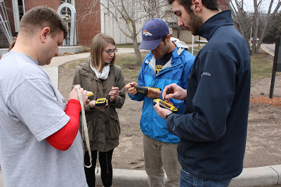
Fig.1. Students and Martin preparing to gather ground control points.
They used varied equipment to gather the data points
including; Nomad, Juno and Topcon units. 

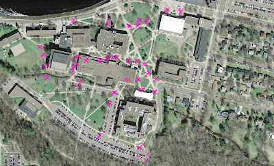
Fig.2. The data point gathered by students were loaded into Arcmap as a
feature class to be used to georeference our aerial images.

The cylinder of helium was successfully transported from storage on the second floor, down one floor and around the Phillips Science Building to the garage without incident (figure 3) where it was used to fill a large balloon. The balloon is the source of elevation for the mapping rig. It is controlled from the ground by operators tethered to the balloon and camera using several hundred feet of cord.

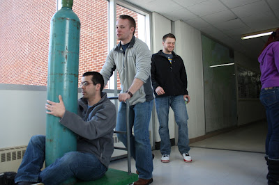
Fig.3. Transportation of the helium from storage to the shed where it was
used to fill the balloon.

Approximately 700 feet of tether cord were measured out and marked in 50 foot sections (figure 4) so we could track the amount of cord being used and the approximate height of the balloon rig. This cord was then fastened to the base of the balloon.

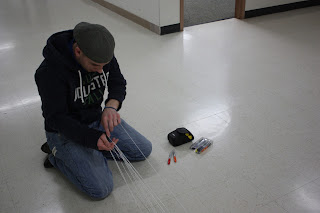
Fig.4. Students measured 700 feet of cord used to guide
the mapping rig  in 50 foot sections.

Our previous experience taught us that the foam box (figure 5) was not a very stable platform to photograph from so we went back to the bottle design we originally planned for, but using a fan I found these were also very unstable in the wind and got tossed and spun a lot. To stabilize the rig I used an old aluminum arrow that I had (the aluminum is strong and lightweight) and fixed a vertical wing or blade to one end. Then I cut the arrow shaft to the bottle length and wrapped the ends good with electrical tape so they would not damage the balloon. When this blade was added to the bottle (figure 6), it was sufficiently stabilized. Both the amount of spin and the amount of roll/bounce were reduced greatly. When it was time to assemble the rig we were wary of how well the camera was mounted inside the bottle and were afraid it might come loose. It had been suggested to try to mount the camera directly to the bottom of the bottle but this, I believe, would have also been unstable due to the movement of the balloon. To securely fasten the camera and isolate it from the roll of the balloon we decided to mount the camera directly to the arrow shaft and loose the bottle. The bottles main function was to help protect the camera in the event of a collision with the ground or another object so now we had to be more careful with the rig. We mounted the camera using cable ties and tape and made sure we could set the controls and operate it with it mounted. We used cordage tied to both the front and back ends of the arrow shaft to suspend the rig from the balloon (figure 7). By keeping the mounting points of the cord as far apart as possible we hoped to make the rig more stable. We found the center of balance in the rig and tied an overhand knot in the cord giving us a loop to mount the rig from, and used a karabiner to fasten the rig to the balloon.

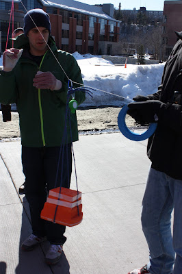
Fig.5. The original foam box used during our first attemt
at mapping was not a stable platform so it was not used.

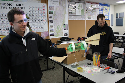
Fig.6. The bottle rig was stabilized using a fin and attached using an arrow shaft.

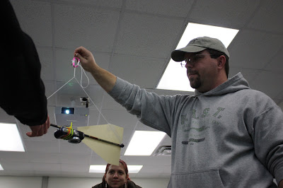
Fig.7. We eventually scrapped the bottle rig due to concerns
over how well the camera was fastened into it. The result was
the fin with the camera attached directly to the shaft.

After the rig was fully assembled we brought it to the UWEC campus mall area. This is a large, very open area great for the initial launch. We set the camera to take continuous images, double checked the rig and proceeded to launch the rig. We let out cord to get to an elevation of 400 feet above the ground, during this time we lost count of how much cord had been released and had to estimate that we were at least to 400 feet. We guided the balloon rig across the campus mall, around the Davies building and east across the parking lot. Then we came back and around the Phillips building and out to the street. We proceeded north through lower campus to the foot bridge and across the Chippewa River and on to Water street. We then guided the balloon west on Water Street to 2^nd avenue then crossed south into the Haas parking lot. After crossing the lot we were forced to bring the rig in due to overhead obstructions (trees). At this point we found that the rig was approximately 500 feet in the air. We walked the rig back to the south end of the foot bridge where we redeployed it. Now we guided it east on Garfield avenue to the steps that climb to upper campus. The balloon rig was guided up the steps and to the south/west through upper campus. Near the upper campus recreation area the balloon was again retrieved (figure 8). After retrieving the rig we found the camera battery almost dead and almost 5000 images on the SD card. The images were loaded into the computer system for later use.

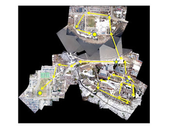
Fig.8. These are the routes we used to guide the mapping rig
around campus, the arrows are indicating the direction of travel.
The stars indicate areas of rig deployment, while the
 circles indicate the area where the rig was brought down.

To process the pictures I first had to go through them to find suitable pictures for mosaicing. I looked for photos which were well focused, and not washed out (figures 9,10). Then I chose photos that covered the area of interest and overlapped each other by at least 50 – 60%. The reason for this is the pictures are best in the center 1/3 and become more distorted as you move to the edges. By overlapping the images we can maintain as much of the centers of the images as possible. Then in Arcmap we open a new file geodatabase and open new map document. I set the document workspace environments to the new geodatabase, and opened the georeferencing toolbar. We split the class into six groups, each group was to georeferenced a specific portion of campus to minimize the amount of time each student would spend referencing the photos. My groups area was the around the Haas Fine Arts Center, north of the Chippewa River on lower campus. To georeference the photos we have to start with some sort of ground data to reference them to. We did not have any ground control points collected in the area we were working on so I used two other sources. The first was a .tif image of the entire campus area, pre-construction (the campus has undergone a lot of new construction over the last couple of years), the second was a layer file that was built from a CAD file containing the true locations of all the buildings on campus. I used both of these but to make the building locations more usable I used a polygon to vertices tool to create vertices of the buildings (fugure11). While referencing the photos I could now snap right to a building corner as a ground control point (GCP). For each photo I began by adding the photo to the workspace and zooming to the photo layer, selecting the photo in the georeferencing toolbar, and selecting the GCP tool from the toolbar. The GCP’s selected had to be points that were easily identifiable and had not changed over time, the building corners, streetlights and lampposts worked well for these.      I then selected a prominent feature such as a building corner as a GCP and zoomed to the building layer where I could locate the corresponding corner in the layer and select it. After I made two GCP’s the photo would be loosely aligned in the image, from here I would make several more choices for good GCP’s to at least 12 points. After reaching 12 points on a photo I changed the method from a first order polynomial to a second order polynomial, helping to smooth out the transition between images. As I added GCP’s to the images I would keep watch on the RMS error. This is root mean square, and is a measure of how accurately the photos are aligned. Ideally I would look for the RMS to be at or below 0.05, but for many of the images it was between 0.05 and 1.00.

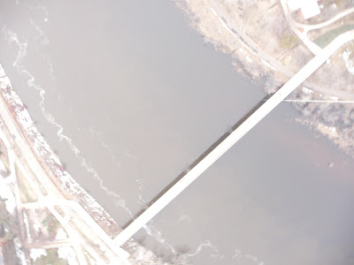
Fig.9. Some of the images were washed out. This was due to the image being
mainly over the water which has low reflectance, the low reflectance causes
 the camera shutter to remain open for an extended period of time.

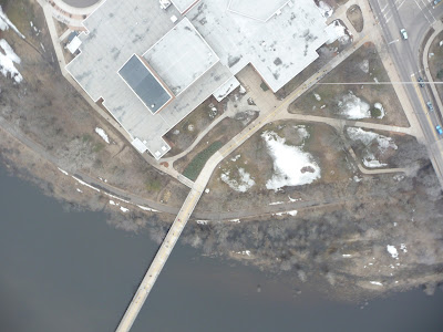
Fig.10. This photo has much better contrast in comparison to the photo in
figure 9. 

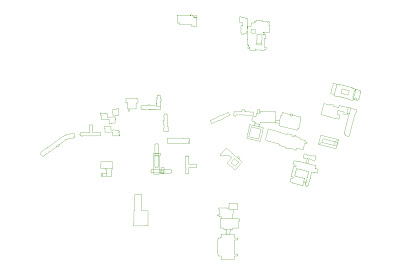
Fig.11. This is a jpeg of the UWEC building vertices created from
the CAD file.

While referencing the photos we had to try to eliminate the cord that the rig was attached to (figure 12). This cord was visible in many of the images. To overcome this I layered the photos beginning in the south/east corner of the area and moving to the west. After reaching the farthest west images I returned to the eastern edge slightly north of the first images and worked to the west again. This process layered the images in such a fashion that the string was removed from all but the most western and northern images (figure 13).

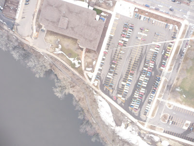
Fig.12. The cord used to guide the balloon rig is clearly visible in the upper right
portion of this photo. While georeferencing the images care was used to
eliminate as much of this as possible.

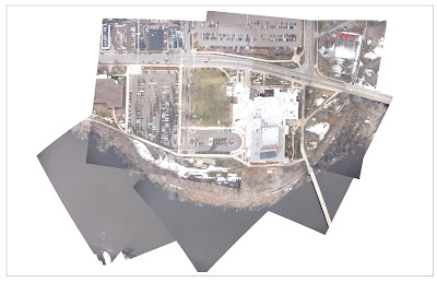
Fig.13. The area north of the foot bridge on lower UWEC campus. Many of
the cord images have been covered by layering; however, near the top and
the right there were no more images to layer leaving the cord visible. 

After completing the area north of the foot bridge I was not happy with how some of the buildings appeared. The roads and other hard ground lines appeared well but in the process the roof of the buildings would become severely distorted. To overcome this I found images with the entire roof in it, I cropped the image to just the roof then referenced it into the image.

Now I could run the mosaic to new raster tool creating a single raster image, and save the image as a .tif in my folder then import the image into my geodatabase (figure 14). After gathering images for the rest of campus and projecting them the same there was a new challenge. The .tif images come with a large area of no data surrounding the image, we have to remove this to mosaic the individual areas of campus together. In the workspace I used create new feature class to create a polygon of the .tif image, then began an editing session to build the polygon around the image and save the edits before quitting the editing session. Then I was able to run the extract by mask tool to crop the image back to the usable portion. After doing this for each of the areas of campus I was able to georeference the areas just as I had the single photos. There were a few spots that needed additional work by adding a few new photos. After referencing all of campus together I ran the mosaic to new raster tool again to get a single complete image of UWEC campus (figure 15).

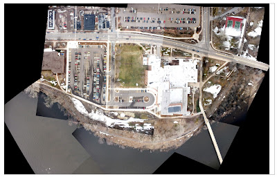
Fig.14. This is the .tif image of the mosaiced area north of the foot bridge on
UWEC lower campus. To mosaic this image with the rest of campus I created
 a new feature class polygon and edited it to the outline of the image within
the .tif, then cropped the image using the polygon and the extract by mask tool.

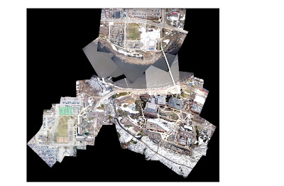
Fig.15. This .tif image shows the area of the UWEC campus that
was photographed. This image is the result of cropping
each of the individual areas, georeferencing them and
mosaicing them together. 

Discussion:

Overall this attempt at balloon mapping went much smoother than the first. The wind speeds were very low allowing us to get the balloon high enough to sufficiently cover the area (figure 16). The images were much improved with the combination of camera rig and lower wind speeds (figure 17). The blade behind the camera kept the rig facing into the wind which minimized the amount of side to side movement in the rig. Without the bottle we could shorten the arrow shaft of the blade to only be slightly longer than the camera and blade, this would eliminate the rig catching up against the tether cord when the rig is deployed.  There also may have been some discrepancy in the height at which we took the images; after we brought the rig in the first time we found that we had overshot our height by at least 100 feet, I am not sure we got back to the same height after we redeployed the rig at the south side of the foot bridge. There is some variation in cell size among the images. Most of the images on lower campus have a cell size between 0.044 and 0.05 meters; however, on Garfield avenue heading east (after redeployment) the image cell size increases to one meter and then on upper campus the cell size is about 0.07 meters. I am not sure what is causing this variation, there may be some variation in rig height. There is also an area east of the nursing building that does not fit together well I believe this is due to cell sizes and bad coverage in the area. Many, not all, of the images in this area do not have much overlap so the edge distortion is very high resulting in poor image matching. It has also been suggested that we make another attempt with a camera that has higher resolution and to stop midway and swap out batteries and memory cards.

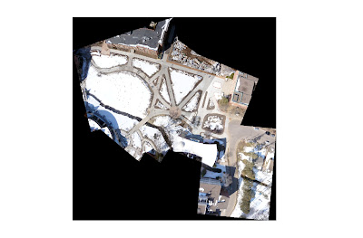
Fig.16. The .tif image from our first attempt to balloon
map. There was a great deal of camera bounce and
swing due to the wind. Also compare the photo coverage
with the photo coverage in figure 17.

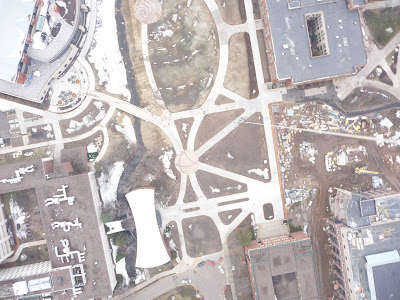
Fig.17. Due to better conditions outside we were able to get a much
greater altitude with our balloon rig. A single image covers the area
of at least two images from the first attempt.

Conclusion:

Although we were quite successful I would like to see another attempt. This has been a trial and error exercise with us learning as we go. We are getting the bugs worked out and are beginning to see some quality to the work. I also fully believe this could work well for large scale, high resolution mapping given the area is free from overhead obstructions. A more comprehensive and accurate set of ground control points would also aid in the process, but we are learning as we go and making continuous improvements.